Topic 4.3 - 数据分组统计
1. 数据分组统计基础
(1) 数据分组统计的概念
数据分组统计,其实就是我们常说的计算均值、方差、标准差等统计量,只不过我们此时不是在整个数据框上计算这些指标,而是在每一组内计算这些指标。
我们来通过以下例子来看一下分组统计的概念:

-
在这个表中,如果我们对全部数据进行求和,得到的结果就是这 9 个销量数字的总和
-
但是如果我们按照不同商品种类进行分组统计的话,我们就会得到每个商品种类的销量总和
-
这个就是分组统计的概念,我们先按照商品种类进行分组,然后在每个组内进行求和,得到每个商品种类的销量总和
(2) 数据分组统计的函数
数据分组统计会用到以下两个重要函数:
group_by()函数:用于对数据框进行分组,里面的参数是列名,按照指定的列名来进行分组-
summarise()函数:用于对分组后的数据框进行统计计算,里面的参数是指标名 = 计算表达式形式,其中计算表达式包括:n():计算每个分组的样本量mean(列名):计算指定列的均值var(列名):计算指定列的方差sd(列名):计算指定列的标准差median(列名):计算指定列的中位数min(列名):计算指定列的最小值max(列名):计算指定列的最大值
这两个函数经常是一起使用的:
- 首先使用
group_by()函数,按照指定的列名来进行分组,然后使用summarise()函数对分组后的数据框进行统计计算,计算出我们想要的指标 - 如果只使用
group_by()函数的话,得到的结果只是一个和原来数据框一模一样的数据框,只不过 R 会记住,这个数据框有个分组的属性,是按照某一列来分组的 - 之后,
summarise()函数计算的结果是一个新的数据框,其中的每一行对应一个分组,每一列对应一个指标
(3) 数据分组统计的示例
我们先导入上一节的包和数据:
library(tidyverse)    # 包含了 ggplot2、dplyr、tidyr 等常用数据处理和可视化包
library(scales)       # 包含用于坐标轴格式化和转换的函数
library(ggokabeito)   # 包含色盲友好的调色板(可选)
library(ggthemes)     # 包含额外的 ggplot 主题
library(patchwork)    # 用于组合多个 ggplot 图形
library(stringr)      # 包含一致的字符串操作函数
library(RColorBrewer) # 包含用于定性和顺序颜色调色板的函数
# 导入 ASX 200 的数据,并且只筛选本节会用到的列
asx_200_2024 <- read_csv("asx_200_2024.csv") |>
  select(gvkey, conml, fyear, ebit, invested_capital, industry)

# 展示数据的前 10 行,来看看数据的结构和内容
asx_200_2024 |> slice_head(n = 10)
| gvkey <chr> | conml <chr>            | fyear <dbl> | ebit <dbl> | invested_capital <dbl> | industry <chr>                                    |
|-------------|------------------------|-------------|------------|------------------------|---------------------------------------------------|
| 013312      | BHP Group Ltd          | 2024        | 22771.0    | 69838.0                | Metals & Mining                                   |
| 210216      | Telstra Group Limited  | 2024        | 3712.0     | 34320.0                | Diversified Telecommunication Services            |
| 223003      | CSL Ltd                | 2024        | 3896.0     | 31584.0                | Biotechnology                                     |
| 212650      | Transurban Group       | 2024        | 1132.0     | 31864.0                | Transportation Infrastructure                     |
| 100894      | Woolworths Group Ltd   | 2024        | 3100.0     | 22292.0                | Consumer Staples Distribution & Retail (New Name) |
| 212427      | Fortescue Ltd          | 2024        | 8520.0     | 24931.0                | Metals & Mining                                   |
| 101601      | Wesfarmers Ltd         | 2024        | 3849.0     | 19863.0                | Broadline Retail (New Name)                       |
| 226744      | Ramsay Health Care Ltd | 2024        | 938.7      | 16465.6                | Health Care Providers & Services                  |
| 220244      | Qantas Airways Ltd     | 2024        | 2198.0     | 6885.0                 | Passenger Airlines (New name)                     |
| 017525      | Origin Energy Ltd      | 2024        | 952.0      | 12867.0                | Electric Utilities                                |
我们首先来看一个例子,我们在上一节的 returns 数据框中,先按照行业来分组,之后计算每个行业中有多少个公司:
returns_summary_obs <- returns |>
  # 按照行业进行分组
  group_by(industry) |>
  # 计算每个行业的观测值数量
  summarise(obs = n()) |>
  # 按照观测值数量从多到少排序
  arrange(desc(obs))

returns_summary_obs
| industry <chr>                                        | obs <int> |
|-------------------------------------------------------|-----------|
| Metals & Mining                                       | 42        |
| Specialty Retail                                      | 14        |
| Construction & Engineering                            | 11        |
| Hotels, Restaurants & Leisure                         | 11        |
| Oil, Gas & Consumable Fuels                           | 9         |
| ...                                                   | ...       |
| Gas Utilities                                         | 1         |
| Independent Power and Renewable Electricity Producers | 1         |
| Multi-Utilities                                       | 1         |
| Pharmaceuticals                                       | 1         |
| Real Estate Management & Development (New Code)       | 1         |
我们再来看一个例子,这时我们只关注几个主要的行业,来看看这些行业的投资回报率 roic 的均值与标准差:
# 定义一个包含主要行业名称的向量
big_industries <- c(
  "Metals & Mining",
  "Specialty Retail",
  "Construction & Engineering",
  "Hotels, Restaurants & Leisure",
  "Oil, Gas & Consumable Fuels",
  "Commercial Services & Supplies",
  "Food Products"
)

# 分组统计每个行业的投资回报率均值与标准差,并且按照均值从高到低排序
returns_summary_stats <- returns |>
  # 只保留选定行业的行
  filter(industry %in% big_industries) |>
  # 按行业分组
  group_by(industry) |>
  # 计算每个行业的投资回报率均值与标准差
  summarise(
    ave_roic = mean(roic, na.rm = TRUE) |> round(4),  # 计算投资回报率的均值,并且保留四位小数
    sd_roic = sd(roic, na.rm = TRUE) |> round(4),    # 计算投资回报率的标准差,并且保留四位小数
    sk_roic = moments::skewness(roic, na.rm = TRUE) |> round(4) # 计算投资回报率的偏度,并且保留四位小数
  ) |>
  # 按照均值从高到低排序
  arrange(desc(ave_roic))

# 显示统计结果
returns_summary_stats
| industry <chr> | ave_roic <dbl> | sd_roic <dbl> | sk_roic <dbl> |
|------------------------------------|----------------|---------------|---------------|
| Construction & Engineering | 0.1442 | 0.0597 | 1.2984 |
| Specialty Retail | 0.1400 | 0.0810 | 0.8255 |
| Commercial Services & Supplies | 0.1332 | 0.0950 | 1.0611 |
| Food Products | 0.0714 | 0.0413 | 0.2335 |
| Metals & Mining | 0.0357 | 0.1770 | -1.5593 |
| Hotels, Restaurants & Leisure | 0.0349 | 0.2012 | -1.9093 |
| Oil, Gas & Consumable Fuels | -0.0028 | 0.1270 | 0.6606 |
对于上面计算出来的偏度,我们还可以使用箱式图来验证:
returns_big_industries <- returns |>
  # 只保留选定行业的行
  filter(industry %in% big_industries) |>
  # 将行业名称设置为因子类型,并且按照均值从高到低
  mutate(industry = factor(industry, levels = returns_summary_stats$industry))
box_plot <- returns_big_industries |>
  # 绘制箱式图,x 轴是行业,y 轴是投资回报率 roic,填充颜色根据行业进行区分
  ggplot(aes(x = industry, y = roic, fill = industry)) +
  # 使用 geom_boxplot 函数绘制箱式图,并且去掉图例
  geom_boxplot(show.legend = FALSE) +
  # 使用色盲友好调色板
  scale_fill_okabe_ito() +
  # 设置图表的标题和轴标签
  labs(
    x = NULL,
    y = "ROIC",
    title = "Return Distribution across Major Industries",
    subtitle = "200 Largest ASX Companies in 2024"
  ) +
  # 默认主题使用 theme_minimal()
  theme_minimal() +
  # 主题中设置以下调整:调整 x 轴文本的角度为 45 度,并且设置水平对齐方式为 1(右对齐)
  theme(axis.text.x = element_text(angle = 45, hjust = 1)) +
  # 允许 x 轴标签换行,设置每行最多显示 15 个字符,这样当行业名称过长时可以自动换行,避免重叠在一起
  scale_x_discrete(labels = scales::label_wrap(15))

# 显示箱式图
box_plot
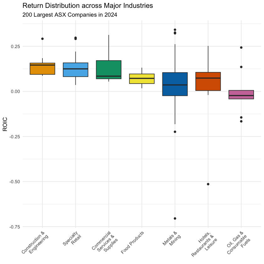
这里我们额外拓展一下:
-
Skewness(偏度)是一个 矩统计量(Moment Statistics),用于衡量数据分布的非对称程度:
- 如果是正数,说明数据是右偏的
- 如果是负数,说明数据是左偏的
- 如果是零,说明数据是对称的
-
而箱式图中的各个指标,都是顺序统计量(Order Statistics):
-
虽然它们都能反应数据分布情况,但是大家要知道它们的本质是不一样的
2. 数据框列操作的进阶操作
事实上,数据分组还可以按照多个指标来进行分组统计。
我们通过以下例子来看看这个概念:
- 在这个表中,我们计算分组销量综合的时候,是按照种类和年份两个变量来分组统计的
- 按照商品种类是 3 类,按照年份是 2 类,所以总共有 3 × 2 = 6 个分组,每个分组对应一个销量综合的数值
在 group_by() 函数中,我们只需加入更多的列名参数,就可以按照多个指标来进行分组统计了:
-
例如,我们在
returns数据框中,先多加一个指标invested_size:- 如果
invested_capital大于 2000 的话,就分为large,否则分为small -
这里我们使用
if_else()函数来实现这个条件赋值if_else()函数的参数是条件表达式、条件为真时的值、条件为假时的值- 按照我们的需求,这个条件赋值可以写为
if_else(invested_capital > 2000, "large", "small")
- 如果
returns_with_size <- returns |>
  # 创建一个新的列 invested_size,根据 invested_capital 的值进行条件赋值
  mutate(invested_size = if_else(invested_capital > 2000, "large", "small"))

returns_with_size |> slice_head(n = 10)
| gvkey <chr> | conml <chr> | fyear <dbl> | ebit <dbl> | invested_capital <dbl> | industry <chr> | roic <dbl> | invested_size <chr> |
|-------------|------------------------|-------------|------------|------------------------|-------------------------------------------------------|------------|---------------------|
| 013312 | BHP Group Ltd | 2024 | 22771.0 | 69838.0 | Metals & Mining | 0.32605458 | large |
| 210216 | Telstra Group Limited | 2024 | 3712.0 | 34320.0 | Diversified Telecommunication Services | 0.10815851 | large |
| 223003 | CSL Ltd | 2024 | 3896.0 | 31584.0 | Biotechnology | 0.12335360 | large |
| 212650 | Transurban Group | 2024 | 1132.0 | 31864.0 | Transportation Infrastructure | 0.03552599 | large |
| 100894 | Woolworths Group Ltd | 2024 | 3100.0 | 22292.0 | Consumer Staples Distribution & Retail (New Name) | 0.13906334 | large |
| 212427 | Fortescue Ltd | 2024 | 8520.0 | 24931.0 | Metals & Mining | 0.34174321 | large |
| 101601 | Wesfarmers Ltd | 2024 | 3849.0 | 19863.0 | Broadline Retail (New Name) | 0.19377738 | large |
| 226744 | Ramsay Health Care Ltd | 2024 | 938.7 | 16465.6 | Health Care Providers & Services | 0.05700977 | large |
| 220244 | Qantas Airways Ltd | 2024 | 2198.0 | 6885.0 | Passenger Airlines (New name) | 0.31924473 | large |
| 017525 | Origin Energy Ltd | 2024 | 952.0 | 12867.0 | Electric Utilities | 0.07398772 | large |
-
之后,我们就有两个分组变量了:
- 一个是
industry,一个是invested_size - 我们就可以按照这两个变量来进行分组统计了
- 一个是
returns_summary_size <- returns_with_size |>
  # 只保留选定行业的行
  filter(industry %in% big_industries) |>
  # 按照行业和投资规模进行分组
  group_by(industry, invested_size) |>
  # 计算每个分组的投资回报率均值
  summarise(ave_roic = mean(roic, na.rm = TRUE) |> round(4)) |>
  # 按照均值从高到低排序
  arrange(industry, desc(ave_roic))

returns_summary_size
| industry <chr>                 | invested_size <chr> | ave_roic <dbl> |
|--------------------------------|---------------------|----------------|
| Commercial Services & Supplies | small               | 0.1681         |
| Commercial Services & Supplies | large               | 0.1070         |
| Construction & Engineering     | small               | 0.1500         |
| Construction & Engineering     | large               | 0.0863         |
| Food Products                  | small               | 0.0714         |
| Hotels, Restaurants & Leisure  | large               | 0.1326         |
| Hotels, Restaurants & Leisure  | small               | -0.0466        |
| Metals & Mining                | large               | 0.0683         |
| Metals & Mining                | small               | 0.0188         |
| Oil, Gas & Consumable Fuels    | large               | 0.0779         |
| Oil, Gas & Consumable Fuels    | small               | -0.0432        |
| Specialty Retail               | large               | 0.2000         |
| Specialty Retail               | small               | 0.1237         |
3. 数据分组统计小结
在 dplyr 包中,数据分组统计主要使用 group_by() 和 summarise() 这两个函数来实现:
-
group_by()函数:- 用于对数据框进行分组,参数是列名,按照指定的列名来进行分组
- 可以按照一个或多个列名来进行分组,如果按照多个列名来分组的话,得到的结果就是按照这些列名的组合来进行分组的
-
summarise()函数:-
用于对分组后的数据框进行统计计算,参数是指标名 = 计算表达式形式
-
常用的计算表达式包括:
n():计算每个分组的样本量mean(列名):计算指定列的均值var(列名):计算指定列的方差sd(列名):计算指定列的标准差median(列名):计算指定列的中位数min(列名):计算指定列的最小值max(列名):计算指定列的最大值
-